Recent work on EMA methods at IPS Munich

Recent work on EMA methods at IPS Munich

Phil Hoole

hoole at phonetik.uni-muenchen.de

1. Comparison of AG501 and AG500

We have used the AG501 in numerous experiments since autumn 2012 We have not done any extensive comparisons of the accuracy of AG501 vs. AG500; however, we report below some statistics taken firstly from information provided by the standard calibration procedure, and secondly from analysis of sensor-stability at the output of our head-movement correction procedures.

The most striking difference since starting to work with the AG501 is that the complicated procedures detailed in Hoole & Zierdt (2010) and online at http://www.phonetik.uni-muenchen.de/~hoole/articmanual/index.html for detecting, and sometimes fixing, instabilities in the calculated positions have become almost irrelevant. This has resulted in enormous savings in the amount of time needed to process the data after the experiment.

One typical observation relating to instabilities in the AG500 was that problems were more likely to occur when the sensor-orientation was close to vertical (i.e. elevation angle close to +/- 90 deg.). This meant that, for example, we always glued the jaw sensor with the main axis of the sensor parallel to the left-right axis rather than parallel to the vertical axis even though the latter arrangement gives more information since one of the main rotational degrees of freedom of jaw movement can then be extracted directly from the sensor orientation coordinates 1 . Since using the AG501 we have routinely been using this vertical orientation and have never encountered any problems. Similarly, for the tongue-tip the most informative orientation of the sensor is parallel to the midline of the tongue (see Hoole & Zierdt, 2010), but with the AG500 it was clearly the case that there was less risk of unstable data if it was attached with the main axis of the sensor at right-angles to the midline (the tongue-tip is so mobile that with the parallel-to-midline arrangement there are many sounds in which the sensor may be pointing vertically up or down). Once again, we have routinely used the parallel-to-midline arrangement for the AG501 without encountering problems.

1.1 Quantitative comparison of AG500 and AG501: (1) Calibration data

The standard calibration procedure provides for each sensor two simple measures that give a rough estimate of calibration quality, referred to as delta_z and stddev_z (see e.g. p. 9 in the current version of the manual ag501-cs5cal.pdf). The circal calibration device acquires data on a plane in which (ideally) the vertical (z) coordinate does not change. Thus any change in the z-coordinate as the circal device rotates through 360 degrees represents error (assuming perfect mechanical accuracy of the circal device itself). ‘delta_z’ simply means the difference between the maximum and minimum z values occurring during the calibration run; stddev_z is the standard deviation of the z coordinates. Clearly both these values should be as small as possible.

We analyzed these values for the calibrations carried out in preparation for about 40 experimental sessions each for AG500 and AG501, giving a total of about 500 sensors for each system.

The following table gives the mean and 95%-ile values for delta_z and stddev_z split by system.

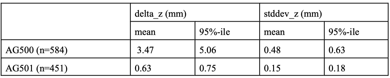
Clearly the values for the AG501 are substantially lower than those for the AG500.

Probably the 95%-ile value, as a measure of the range, is of more practical value than the mean, i.e. 95% of the data have values lower than the values given in the table.

For the AG501 the 95%-ile for delta_z lies only about 0.1 mm above the mean value, indicating that the delta_z value is very stable across a wide range of sessions and sensors. For the AG500 the increase is far greater, of the order of 1.5mm. Similarly, for stddev_z the 95%-ile lies much closer to the mean for the AG501 than for the AG500.

Clearly, this analysis of the calibration data does not constitute a rigorous accuracy test: first because the tests are based on the same data used for the calibration in the first place, and second because only a single plane out of a five-dimensional measurement space is taken into account. Nevertheless, because the delta_z and stddev_z values are readily available we believe that in particular the 95%-ile range is useful for practical work (given that the results above are based on quite a substantial dataset): Sensors for which the values exceed the 95%-iles given above should probably be regarded as potentially unreliable. The results make clear that for the AG500 even quite a substantial amount of distortion in the z-coordinate (around 5mm for delta_z) still has to be regarded as ‘typical’ behaviour, whereas it is possible to be much more restrictive for the AG501.

1.2 Quantitative comparison of AG500 and AG501: (2) Stability of head-movement correction

For this test we looked for a simple way of comparing the performance of the systems during the actual acquisition of experimental data; in particular we wanted a test that could be applied to as much of our available AG500 and AG501 data as possible.

The rationale was a follows:

Following correction for head-movement the coordinates of the sensors used to calculate the adjustment should be constant. However, this will not be the case if there are inaccuracies in any of the sensors used to capture head position. Since the number and location of sensors we use as reference sensors varies somewhat from one experiment to another (depending on our estimate of the quality of the sensors avaiable (see Hoole & Zierdt, 2010, and further remarks below)), we based the following test only on the nose sensor, since this is used in virtually all sessions 2 .

For each session we calculated its average position (just x, y, z coordinates i.e. ignoring the angular coordinates) and then used the root mean square distance from the average value as a measure of stability in the given session.

The following table is based on about 40 recording sessions each for AG500 and AG501. For each session the rms distance from the mean was calculated for each trial, and then the mean and standard deviation of this value over the trials in the session was calculated. The table in turn reports the means and 90%-ile over all sessions

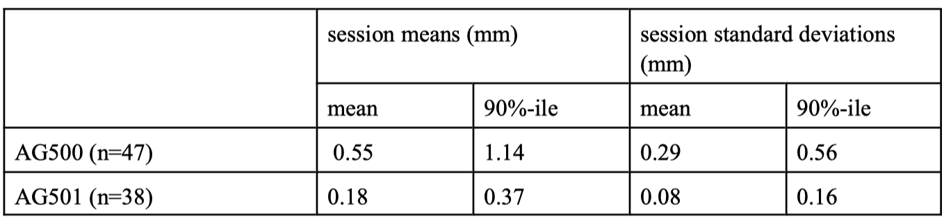
Clearly, once again much lower values are found for the AG501, indicating that correction for head movement is probably much more precise in the newer system.

In fact, the results are in a sense biased in favour of the AG500 since the AG501 dataset included data from a group of seven young children (about age 6), who certainly moved around a lot more in the measurement field than most of the adult subjects, providing quite a challenge for the head correction algorithm (for the AG500 we never recorded any children). In addition, the AG501 dataset included one adult subject who was explicitly asked to behave like a very fidgety subject, and move around a lot during the recordings. For five of these seven children and for the “restless” adult subject the results were at the upper end of the range for the AG501, i.e. close to the 90%-ile values given in the table. But note that the 90%-ile values for the AG501 are still well-below the mean values of the AG500.

See the following link for movies of a representative trial of the “restless” subject:

www.phonetik.uni-muenchen.de/~hoole/articmanual/ag501/

2. Factoring out head movement

The fact that the AG501 seemed to be giving much more stable data provided the impetus to take a fresh look at our procedures for factoring out head movements from speech movements.

Since a minimum of two appropriately positioned and oriented sensors is required to recover all 6 degrees of freedom of head motion, and since it would be disastrous if one of these two sensors were to fail, our usual policy has been to use more than this minimum, typically one on upper incisors, one on bridge of nose, and one behind each ear. Since the distances between sensors rigidly attached to the skull should remain constant over the course of the experiment we would then check the variability of the inter-sensor distances and exclude any noticeably variable sensors from use in the head-correction procedures (see Hoole & Zierdt, 2010, for more background).

This procedure, does not, however, directly tell us how successful compensation for head movement actually is. Since problems with really wild outliers (particularly near the edge of the measurement field) had disappeared in the AG501 we implemented a procedure for quickly estimating the accuracy of head-movement correction for various potential combinations of reference sensors under realistic experimental conditions.

One specific question was the following: Given that our typical four reference sensors basically all give reliable data in the AG501, it is interesting to ask whether using all four actually gives better headmovement correction than the minimum of two. Would it actually be advantageous to simply attach as many spare sensors as possible to the head?

To estimate this under realistic experimental conditions requires a cooperative subject, namely one who can move his head over a wide range of positions and orientations without moving the speech articulators (lips, tongue, jaw).

Then the amount of variability in the articulators after subtracting out head-movement should be zero. In practice one looks for the combination of reference sensors giving lowest variability.

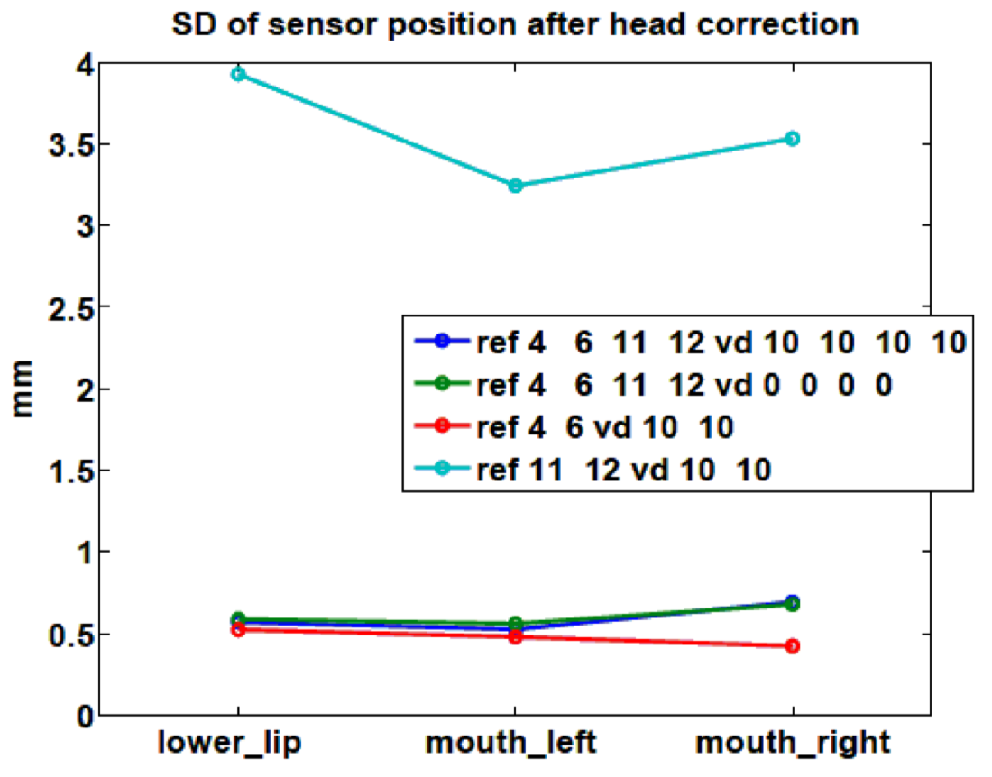
The figure shows the analysis of one such task. The stability after head-correction was analyzed for three sensors attached in the lip region. The different coloured lines show the results for different combinations of reference sensors. The legend gives the numbers of the sensors used (the numbers between ‘ref’ and ‘vd’; the numbers after ‘vd’ will be explained below).

Sensors 4 and 6 were located on the upper incisors and nose; sensors 11 and 12 on the bony prominence behind the left and right ear.

The y-axis shows the amount of variability in sensor position after compensation for head motion (the lower the better).

If we treat the red line as our baseline configuration (i.e. just uses the standard minimum configuration of upper incisors (4) and nose (6)), then it appears that there is no advantage to using the configurations with all four sensors (the dark blue and green lines).

On the other hand, not all combinations of just two sensors are equally good: the light blue line is based on head correction using the sensors behind the left and right ear; clearly it gives much poorer results than any of the other combinations shown here. This may be simply because these sensors are relatively far away from the mouth and lip sensors. For example, the effects of any imperfections in extracting the pitch angle of the head (rotation about the left-to-right axis) would be magnified with increasing distance from the reference sensors.

The procedure outlined here can be applied to any experimental session where the subject is able to record at least one trial with a wide range of head positions, while keeping the speech articulators immobile. The result shown here has turned out to be fairly typical, i.e. if the upper incisor and nose sensors are available then there has not appeared to be any obvious advantage in using additional sensors in the head correction. But in any given session, there is always the possibility that one of these two preferred sensors may malfunction, in which case it is useful to have a principled way of choosing an alternative combination of sensors.

Illustrative movies for the extraction of head movement (for the “restless” subject mentioned in section 1.2 above) can be found here:

www.phonetik.uni-muenchen.de/~hoole/articmanual/ag501/

A note on the concept of ‘virtual sensors’

Our algorithm for head movement correction uses the concept of ‘virtual sensors’ as a means of using position and orientation information simultaneously when determining the six degrees of freedom of head movement. Basically, the azimuth and elevation coordinates are used to define the position of a ‘virtual sensor’ at a fixed distance from the main sensor. As discussed in Kroos (2009) this requires a somewhat arbitrary decision as to the appropriate distance to use (larger distances effectively weight the orientation information more strongly). In the past we had used a fixed value of 50mm, because, very roughly, this seemed to give virtual sensor coordinates with about the same level of noise as the actual measured sensors. As part of the developments described here we took the opportunity to investigate more systematically how the value chosen for the virtual distance affected the quality of the head-movement correction.

Briefly, the conclusions were as follows:

(1) A lower value appears preferable: 10mm gives a good results, there was no evidence that 50mm gives better results than 10mm, and increasing the distance beyond 50mm starts to result in less stable performance.

(2) When the minimum of two reference sensors is used then solving for the six degrees of freedom of head movement is, of course, only possible if the additional information captured by the virtual sensors is used. However, as soon as more than this minimum of two sensors is available then it is immaterial whether the virtual sensors are used or not (at least as long as the sensors are not collinear, and not clustered too close together). This is illustrated in the figure by the dark-blue and the green lines. For the dark-blue line a virtual-sensor distance of 10mm was used (indicated by ‘vd 10 10 10 10' in the legend), whereas for the green line the virtual sensors were deactivated by setting the distance to 0. The lines are virtually indistinguishable. This fits in with the conclusion above that there is no particular advantage to simply using as much reference-sensor information as possible. Thus the two-sensor (upper-incisor plus nose) solution, with the main axes of the sensors oriented at right-angles to the line joining the two sensors seems to be a very effective arrangement.

3. Filtering

It is an interesting but insufficiently appreciated feature of electromagnetic movement transduction systems like the AG500 and AG501 that they inherently incorporate the possibility to determine the appropriate amount of smoothing to apply to the raw data. Often the choice of cutoff-frequency for lowpass-filtering articulatory data is simply based on some kind of a-priori knowledge or the investigator’s intuition as to what looks plausible. There is certainly always a temptation to oversmooth, because strongly smoothed data at least looks ‘nice’ and may well be superficially easier to analyze.

The key concept for the following remarks is the so-called rms-value that is derived when sensor position and orientation is derived from the raw amplitude data. Because of the redundancy built into EMA systems in which 6 (AG500) or 9 (AG501) transmitter signals are used to solve for the 5 sensor degrees of freedom, then the system will usually calculate a reasonably accurate position, even if there is some distortion in the raw measured amplitude values (some distortion is bound to occur in any real measurement system). The rms-value is in effect an estimate of this distortion: once the system has solved for the set of positions and orientations most compatible with the raw measured amplitudes it can use the magnetic field model to calculate the amplitudes that would be expected for those positions in an error-free system. The difference between the predicted and measured amplitudes gives the rmsvalue.

The basic idea here is that excessive smoothing of the raw data constitutes a kind of distortion, because the smoothed data will no longer faithfully follow fast changes in the data that correspond to the actual articulatory movements. Thus the rms-value can be expected to increase.

The analysis shown here was based on a recording of a trumpet player performing fast tonguing movements (specifically double-tonguing with alternating closures formed by tongue-tip and tonguedorsum, at a rate of about 6 articulations per second for each articulator). Fast speech movements can be expected to show similar properties; the trumpet data just happened to be the most convenient available dataset, since the fast movements were sustained for about 10s, giving ample data for extraction of stable statistics on the rms-values).

[Link to a movie clip showing these tongue movements : www.phonetik.uni-muenchen.de/~hoole/articmanual/ag501/]

The raw amplitudes were filtered with a Kaiser design FIR lowpass filter with cutoff frequency ranging from 5Hz to 100Hz in 5Hz steps 3 . After filtering the positions were calculated for sensors located on tongue-tip and tongue-dorsum, and the 95%-ile of the rms-value was extracted for each sensor at each filter setting. The results are shown in the following figure:

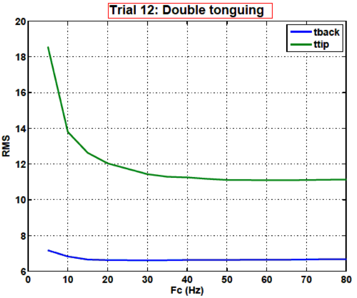
As predicted, RMS goes up as the cutoff frequency decreases. For the tongue-tip the increase in RMS is apparent for all cutoff frequencies below about 40Hz, for the tongue-dorsum below about 20Hz. The reason why there is more high-frequency energy in the tongue-tip signal, even though both articulators were performing cyclical movements at about the same rate (6 per second), is probably that the tonguetip is hitting a harder boundary at closure than the dorsum is. For these cyclical movements the results indicate that there is high-frequency energy in the tongue-tip signal up to about the 6 th harmonic. Note that some speech movements are potentially even faster than those analyzed here: this is of course the case for trills, but may be also the case for taps and flaps.

4. Twin EMA setup

We have implemented a setup for synchronous acquisition from an AG500 and an AG501 system. This was briefly outlined in a presentation at the Cologne convergence workshop (satellite of ISSP 2014):

Links to this presentation and to a movie of twin speaker movements discussed in this presentation: www.phonetik.uni-muenchen.de/~hoole/articmanual/ag501/ Some additional examples of intrusive gestures in the twin-speaker paradigm (and brief discussion of techniques for analyzing entrainment based on EMA data) are given in a presentation at a workshop on entrainment:

http://page.home.amu.edu.pl/?page_id=26

Although the combination of AG500 and AG501 is easy enough to set up (there is no appreciable interference between the systems) for more extensive work we plan to upgrade the old AG500 machine to an AG501 because of the much greater stability of the data in the newer system (particularly important in experimental paradigms where the subjects should be given as much freedom of movement as possible).

References

Hoole, P. & Zierdt, A. (2010). Five-dimensional articulography. In: Speech Motor Control: New developments in basic and applied research, Editors: Ben Maassen, Pascal H.H.M. van Lieshout. OUP, pp. 331-349. http://www.phonetik.uni-muenchen.de/~hoole/pdf/hoole_zierdt_oup_proofs_editable.pdf Kroos, C. (2009). Using sensor orientation information for computational head stabilisation in 3D Electromagnetic Articulography (EMA). In Proceedings of Interspeech 2009. Brighton, UK, (pp. 776–779).