Predicting tongue shapes from a few landmark locations
Predicting tongue shapes from a few landmark locations Chao Qin1 , Miguel ´A. Carreira-Perpi˜n´an1 , Korin Richmond2 , Alan Wrench3 , Steve Renals2 1EECS, School of Engineering, University of California, Merced, USA 2Centre for Speech Technology Research, University of Edinburgh, UK 3Queen Margaret University College, Edinburgh, UK {cqin,mcarreira-perpinan}@ucmerced.edu, korin@cstr.ed.ac.uk, awrench@qmuc.ac.uk,s.renals@ed.ac.uk Abstract We present a method for predicting the midsagittal tongue contour from the locations of a few landmarks (metal pellets) on the tongue surface, as used in articulatory databases such as MOCHA and the Wisconsin XRDB. Our method learns a mapping using ground-truth tongue contours derived from ultrasound data and drastically improves over spline interpolation. We also determine the optimal locations of the landmarks, and the number of landmarks required to achieve a desired prediction error: 3–4 landmarks are enough to achieve 0.3–0.2 mm error per point on the tongue. Index Terms: ultrasound, midsagittal tongue contour, tongue tracking, articulatory database 1. Introduction We consider the problem of reconstructing the shape of the tongue given the location of a few landmarks on its surface. For example, two articulatory databases (Fig. 1), the Wisconsin XRDB (using X-ray microbeam) [1] and MOCHA-TIMIT (using EMA) [2] give the 2D locations of 3–4 metal pellets attached to the tongue tip and dorsum (as well as the locations of the lips and other articulators, and the acoustic wave). Given the location of these pellets at a given time, what does the entire tongue shape look like? In fact, are 3–4 pellets enough to characterise the tongue shape accurately at all? The ability to derive the full tongue shape from a few pellets would allow to animate the tongue shape for visualisation purposes, and could be used as an input to methods for articulatory speech synthesis and inversion. It would also help to determine the optimal number and placem
收录时间:2020-02-05T09:06:45Z
使用资料正文
Predicting tongue shapes from a few landmark locations
Chao Qin1 , Miguel ´A. Carreira-Perpi˜n´an1 , Korin Richmond2 , Alan Wrench3 , Steve Renals2
1EECS, School of Engineering, University of California, Merced, USA
2Centre for Speech Technology Research, University of Edinburgh, UK
3Queen Margaret University College, Edinburgh, UK
{cqin,mcarreira-perpinan}@ucmerced.edu, korin@cstr.ed.ac.uk, awrench@qmuc.ac.uk,s.renals@ed.ac.uk
Abstract
We present a method for predicting the midsagittal tongue contour from the locations of a few landmarks (metal pellets) on the tongue surface, as used in articulatory databases such as MOCHA and the Wisconsin XRDB. Our method learns a mapping using ground-truth tongue contours derived from ultrasound data and drastically improves over spline interpolation. We also determine the optimal locations of the landmarks, and the number of landmarks required to achieve a desired prediction error: 3–4 landmarks are enough to achieve 0.3–0.2 mm error per point on the tongue.
Index Terms: ultrasound, midsagittal tongue contour, tongue tracking, articulatory database
1. Introduction
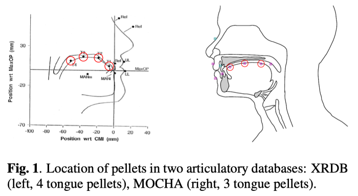
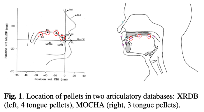
We consider the problem of reconstructing the shape of the tongue given the location of a few landmarks on its surface. For example, two articulatory databases (Fig. 1), the Wisconsin XRDB (using X-ray microbeam) [1] and MOCHA-TIMIT (using EMA) [2] give the 2D locations of 3–4 metal pellets attached to the tongue tip and dorsum (as well as the locations of the lips and other articulators, and the acoustic wave). Given the location of these pellets at a given time, what does the entire tongue shape look like? In fact, are 3–4 pellets enough to characterise the tongue shape accurately at all? The ability to derive the full tongue shape from a few pellets would allow to animate the tongue shape for visualisation purposes, and could be used as an input to methods for articulatory speech synthesis and inversion. It would also help to determine the optimal number and placement of pellets during EMA or X-ray recording.
In this paper, we focus on reconstructing the midsagittal contour of the tongue rather than its full 3D shape, because our ultrasound data is limited to 2D images. However, our approach extends to the 3D case. A simple reconstruction approach (that we and others have used) is to fit a smooth contour (e.g. a cubic or even piecewise linear spline) to the landmarks, justified by the observation that the tongue body is continuous and reasonably smooth during speech. However, smoothness is not enough to characterise the real behaviour of the tongue, which can display very complex shapes during normal speech. For example, its midsagittal contour can show humps or valleys between landmarks or bend significantly in the tip or root (Figs. 2 and 4); and the tongue cannot go through the palate or teeth. It is possible to try to model the tongue shape by having a function with many control parameters and to model compression against the palate or teeth by assuming constant volume, as done in the Baldi talking head [3]. However, setting these parameters is difficult and time-consuming even for an expert, and even un-der the best settings the predicted shape may not look realistic enough. A similar problem arises in computer animation of the human body, where a combination of motion-capture and machine learning are able to reproduce realistic motion.
In this paper, we follow a machine learning approach, where we estimate a nonlinear mapping from the landmark locations to the tongue contour using ultrasound data recorded for a subject during normal continuous speech. With this ground truth, estimating the optimal parameters can be done by numerical minimisation of the reconstruction error, and we find that the predicted tongue contours look very realistic. Our approach is similar to that of [4], who considered inferring midsagittal pharynx shapes from the tongue using MRI data but limited to 11 static vowels and using linear regression. In addition, we can also estimate the optimal location of the landmarks on the tongue, and the number of landmarks we need to achieve a given error. Section 2 describes the data collection, section 3 the predictive model and section 4 the experimental results.
2. Data collection
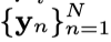
In order to be able to map landmarks to a full tongue contour, we need ground-truth data for tongue contours. Specifically, we consider a dataset consisting (for a given speaker) of N contours is a vector giving the 2D coordinates of each of P points along the tongue. We collected such a dataset from ultrasound recordings.
Tongue contour tracking from ultrasound Unlike EMA and X-ray microbeam, ultrasound technology can image realtime movement of the entire midsagittal tongue contour during speech in a noninvasive and unobtrusive way. Other advantages, such as high temporal resolution, portability and low cost make it very appealing in speech research. Ultrasound has disadvantages as well: the images contain speckle noise and unrelated edges; it does not image passive articulators, only the tongue; and the only image area that is visible is between the thyroid cartilage and the front of the mandible because of shadows; see [9] for a guide on using ultrasound to analyse tongue motion. (Recording ultrasound and EMA simultaneously is difficult due to interference between the two channels, although such a dualchannel database [6] is being investigated.)
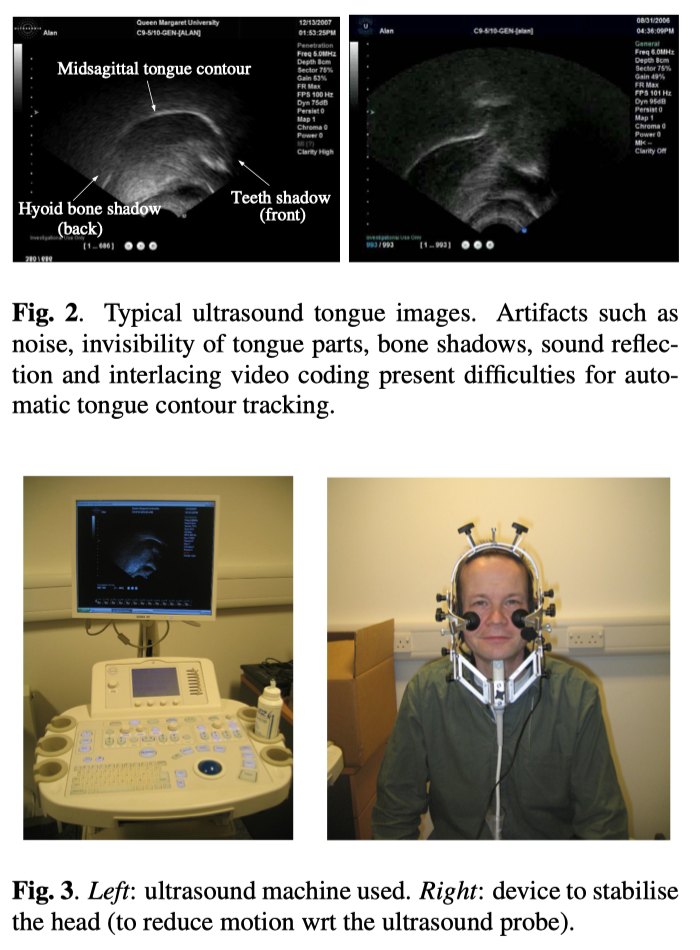
Given a set of 2D ultrasound images of a tongue (Fig. 2 shows two sample images), our goal is to extract the tongue contour (the lower edge of the highlighted strip) from each image. Manual tracking of the tongue contours suffers from several drawbacks well known in biomedical image analysis, including user bias, user fatigue, and not being able to achieve reproducible results. Also, it becomes infeasible for a large number of ultrasound images. Therefore, it is crucial to have an automated system for tongue movement analysis. However, the noisy nature of ultrasound images makes it very difficult to track tongue shapes reliably and automatically (see [5] for a comprehensive survey on ultrasound image segmentation), and this is compounded when dealing with multiple utterances and speakers. Since in our study it was important to obtain highquality ground-truth contours, we adopted a semi-automatic approach: we used a state-of-the-art contour tracking algorithm, which gave us a reasonable tongue contour at each frame, and then we adjusted the contours manually if necessary. We used the automatic tongue contour tracking software EdgeTrak [7]. Its algorithm is essentially based on the active contour algorithm of [8], which iteratively minimises an energy function designed to detect contours of the object in the image. We observed in practice that the algorithm could get stuck at a local minimum and lose track, hence the need for manual corrections.
As discussed, obtaining ground-truth tongue contours is either unreliable (with automatic methods) or time-consuming (with manual methods). Future work should address the issue of adapting a model learned on a dataset (e.g. from one speaker) to a different setting (e.g. a different speaker).
Tongue contour dataset Following the procedure described above, we have created an ultrasound database at Queen Margaret University and the University of Edinburgh. It contains two speakers (one male, maaw0, and one female, feal0) with different Scottish accents. Two data streams were recorded synchronously for each speaker: acoustic waves (which we did not use in this study) and ultrasound videos. The ultrasound recorded the movements of the tongue in the midsagittal plane at 100 Hz. Each speaker recorded a set of 20 British TIMIT sentences designed to be phonetically balanced. In this study, we use data from maaw0, consisting of two parts: one part contains 800 image frames from one utterance (db1); the other part contains 6 000 image frames from 10 utterances but recorded in a separate session (db2).
Although the ultrasound probe is held against the chin while recording, it is possible in principle that the chin and the probe shift with respect to each other during recording. This would require normalising the contours wrt a fixed reference. However, we found this unnecessary for two reasons: in a pilot experiment, we compared the prediction results with normalisation (by shifting the data to zero mean and a given orientation) and without normalisation, and found little difference; in addition, we used a device (Fig. 3) to stabilise the probe wrt the head. Thus, the experiments described here used no normalisation.
3. Predictive model
We define the tongue reconstruction problem as follows. Of the P points along the contour, we choose K (say, 3) to represent the landmarks, or pellets affixed to the tongue (call this vector x ). We then want to predict all P points (or rather, the remaining P − K) using a mapping f(x) = y that we estimate from a training set. We represent f using a radial basis function (RBF) network [10]: f(x) = WΦ(x) with weight matrix W of 2P × M and M Gaussian basis functions
  with µi and width σ. The reason for choosing a RBF network is that, besides being able to approximate many mappings accurately, it also simplifies considerably our computations. We can fix the RBF centres µI once and for all on the basis of the training set of contours
  (e.g. by vector quantisation) and estimate W depending on the choice of landmarks x by solving a linear least-squares problem (without local minima).
As interpolation method (not based on a training set), we use a cubic B-spline (Matlab function spline).
4. Experimental results
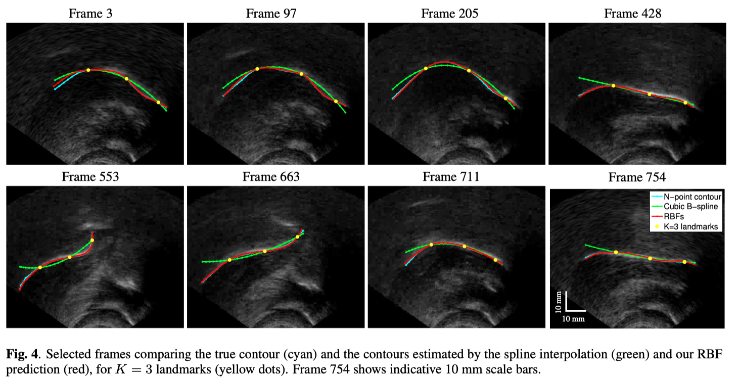
RBF prediction vs. spline interpolation of the tongue contour We trained a RBF network on database db1, with parameters found by cross-validation (M = 110 basis functions fitted by k–means with 10 random initialisations; σ = 20 mm). Fig. 4 compares in selected frames the true tongue contour and the contours estimated by spline interpolation and by our RBF prediction, given K = 3 fixed landmarks (representing 3 EMA pellets). Fig. 4 also illustrates the rather complex shapes that the tongue can adopt, with significant changes in curvature, in particular when raising the tip. The contour predicted by the RBF overlaps almost perfectly with the true contour, so the latter is barely visible. The spline contour often deviates significantly from the true one. For example, since the spline behaves like an elastic bar, it is impossible for it to predict a sharp valley or hump between two adjacent landmarks (frames 97, 205, 553). When the landmarks are aligned (e.g. frames 428, 754) the spline naturally adopts a straight line shape, which is physically infeasible for the tongue, and different indeed from the true contour. In all these situations the RBF prediction works very well. The advantage of the prediction based on a training set is largest when extrapolating beyond the end landmarks, near the root or the tip of the tongue.
Optimal number and location of the landmarks In this experiment, we used database db2. In order to determine the optimal location of K landmarks, we would need to fit a predictor to each of the (pk) combinations (where our contours have P = 24 K points). We limit the computational cost involved as follows. (1) By using a RBF network with fixed basis function centres and width, we only need to estimate the linear weights W for each combination. (2) We ignore unreasonable arrangements of landmarks by dividing the contour into K consecutive segments and constraining each landmark to select points from one; for example, for K = 3, landmarks 1, 2 and 3 can only select points 1–8, 9–16 and 17–24, respectively. This prevents landmarks from being all very close, or very far from each other, which undoubtedly would lead to a much worse prediction. This resulted in 145, 513, 1297, 2501 combinations for K = 2, 3, 4, 5, resp. The number of combinations for K = 6 (4900+) or higher required too much computer time for this study. For each combination, we performed 5-fold cross-validation to choose the optimal parameters and reported the averaged reconstruction errors. The optimal parameters of the RBF network (M, σ) (number of BFs and width in mm) were:

We report the root-mean-square error (RMSE) in mm for each contour point in Fig. 5 (left), where n is the index of the contour in the dataset (with N = 6 000 contours for db2), and
  and
and are the true and reconstructed tongue contours, respectively. Fig. 5 (right) reports the RMSE averaged over the P contour points.
Fig. 5 (left) shows that the prediction errors at each contour point are roughly symmetric around the fixed landmarks, with the lowest (zero) error at the landmarks themselves, and the highest error approximately in the midpoint between landmarks, or at the ends of the contour. The errors are largest at the tip of the tongue, consistent with its movement being the most complex. From Fig. 5 (right), using only 2 landmarks yields an optimal error of 0.6 mm, while using 3 yields less than 0.3 mm and 4 yields 0.2 mm. Using more landmarks yields diminishing returns; it is also practically harder to attach that many pellets to the tongue. The line labelled “worst” is actually not much worse than the optimal, because we have ruled out pellet arrangements that would indeed yield a far larger error (e.g. having all pellets next to each other).
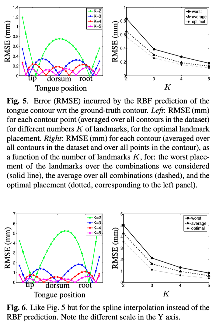
For the spline interpolation, we predicted the contour y by considering a uniform grid of P locations along the X axis (with known Y values for K points) and applying to it the spline function. Consistent with the previous section, the spline interpolation (Fig. 6) is always much worse (by an order of magnitude) than the RBF prediction, although its error improves as K increases.
Fig. 7 shows the optimal location of the landmarks for K = 2 to 5. The landmarks are roughly equidistant along the tongue contour, but somewhat closer to each other near the tongue tip, consistent with the fact that the tongue tip shows more complex movements than the rest of the tongue. The end landmarks are close to the contour ends (tip and back), but not right at the ends. The scale bar allows to determine the positions in mm, and (after rescaling by the total tongue length) one can determine the approximately optimal placement for a different speaker. The approximate locations of the 3 pellets that were used in the MOCHA database are quite close to the optimal ones. From Fig. 5 we then estimate that the tongue contours may be reconstructed from the 3 MOCHA pellets with an error of around 0.3 mm at each point on the tongue contour. The fact that the “worst” and “average” lines in Fig. 5 (right) increase the error by only about 0.1 mm means that, if we cannot place the landmarks optimally as given by Fig. 7, the following recipe will yield near-optimal results: place two pellets 2 to 4 mm from the tongue ends (tip and root, i.e., as far forward and backward as possible), and place the remaining K − 2 pellets so all K pellets are regularly spaced.
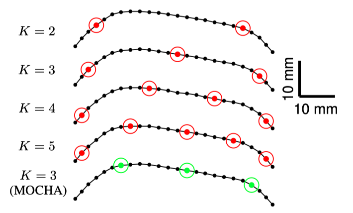
Fig. 7. Optimal location of K landmarks (for K = 2, 3, 4, 5)
depicted on a sample tongue contour (the tip is to the right
and the root to the left). The bottom contour shows the
approximate location of the 3 pellets used in the MOCHA database.
5. Conclusion
We have shown that realistic tongue contours (with errors well below 0.4 mm) may be predicted from as few as 3–4 landmarks (optimally located on the tongue) using a nonlinear mapping learned from ultrasound data. This information may be used to determine the optimal number and locations of pellets for EMA and X-ray microbeam technology. Although our dataset was small and limited to one speaker, the results demonstrate the approach is much more successful than spline interpolation, and quantify the extent to which the EMA/X-ray data is a good representation of the tongue. Future work will involve adapting the model to a different speaker for which we have no (or very little) data; animating tongue contours for vocal tract visualisation of EMA/X-ray databases; and augmenting the tongue represen-tation in data-driven methods for articulatory speech synthesis and articulatory inversion. This will improve our understanding of the limitations of current articulatory databases for articulatory inversion, articulatory synthesis and vocal tract visualisation. The method is also applicable to predicting the 3D shape from landmarks if 3D ground truth is available.
6. Acknowledgements
MACP thanks D. Massaro and M. Cohen (UC Santa Cruz) for useful discussions. Work funded by NSF CAREER award IIS0754089 and Marie Curie Early Stage Training Site EdSST (MEST–CT–2005–020568). The ultrasound data and extracted contours are available from the authors.
7. References
[1] J. R. Westbury, X-Ray Microbeam Speech Production Database User’s Handbook Version 1.0, June 1994.
[2] A. A. Wrench, “A multi-channel/multi-speaker articulatory database for continuous speech recognition research,” in Phonus. Institute of Phonetics, 2000.
[3] M. M. Cohen, J. Beskow, and D. W. Massaro, “Recent developments in facial animation: An inside view,” in Proc. Third Auditory-Visual Speech Processing Conf. (AVSP’98), 1998.
[4] D. H. Whalen, A. Min Kang, H. S. Magen, R. K. Fulbright, and J. C. Gore, “Predicting midsagittal pharynx shape from tongue position during vowel production,” Journal of Speech, Language and Hearing Research 42(3):592–603, 1999.
[5] J. A. Noble and D. Boukerroui, “Ultrasound image segmentation:A survey,” IEEE Trans. Medical Imaging 25(8):987–1010, 2006.
[6] M. Aron, E. Kerrien, M.-Odile Berger, and Y. Laprie, “Coupling electromagnetic sensors and ultrasound images for tongue tracking: acquisition set up and preliminary results,” in Proc. Int. Seminar on Speech Production (ISSP’06), 2006.
[7] M. Li, C. Kambhamettu, and M. Stone, “Automatic contour tracking in ultrasound images,” Clinical Linguistics and Phonetics 19:545–554, 2005.
[8] M. Kass, A. P. Witkin, and D. Terzopoulos, “Snakes: Active contour models,” Int. Journal of Computer Vision 1:321–331, 1988.
[9] M. Stone, “A guide to analyzing tongue motion from ultrasound images,” Clinical Linguistics and Phonetics 19:455–501, 2005.
[10] C. M. Bishop, Neural Networks for Pattern Recognition, Oxford University Press, New York, Oxford, 1995.