
695 阅读 2020-09-27 09:30:04 上传
以下文章来源于 认知语言学
转自微信公众号:量化小白上分记
看多了前面的铺垫,接下来写一写可以实操的。本篇给出写择时策略回测的详细步骤,并用代码展示全过程,代码用python写,数据和代码后台回复“择时”获取,可以自己测试。
择时策略
根据百度百科的解释,择时交易是指利用某种方法来判断大势的走势情况,是上涨还是下跌或者是盘整。如果判断是上涨,则买入持有;如果判断是下跌,则卖出清仓,如果是盘整,可以高抛低吸。
从量化角度来说,择时是通过资产的数据构造出买卖信号,按照买卖信号进行交易。回测就是实现这整个过程。
本文以最简单的双均线策略为例进行回测,具体规则如下:
短均线上穿长均线(金叉),且当前无持仓:买入;
短均线下穿长均线(死叉),且当前持仓,卖出;
其他情况,保持之前仓位;
可以考虑控制回撤,单次亏损超过一定幅度平仓。
回测评价
对于策略的评价,总体分为收益和风险两方面,或者将两者综合起来,列一些最常用的评价指标。
年化收益
回测起点到终点的累积收益年化,算复利或单利都可以,复利假设策略的盈利也会被用于投资,因此复利算出来结果会更好看一些。
夏普比
夏普比 = (策略期望收益率 - 无风险收益率)/策略波动率
夏普比综合衡量了收益和风险,是最广泛应用的指标。
胜率
统计胜率要先统计交易次数,然后计算所以交易中盈利次数占的比例
最大回撤率
回撤是策略从前期最高点到当前时点的亏损,最大回撤是所有回撤中的最大值,反映的是策略的最大可能损失。
单次最大亏损
所有单次交易中的最大亏损
策略阶段性表现
对策略时间段进行分割,统计每个时间段内上述指标的变化情况,本文按年进行分割,统计测年逐年的收益率和相对于基准的超额收益率。
其他
除此外,还有波动率、下行风险、索提诺比率等各种指标,python中有专门的模块可以计算各种指标,这里我们自己算出各种指标,供参考。
此外,还需要测试策略的稳定性,对策略中参数进行扰动,检验策略的敏感性情况,好的策略应该是参数不敏感的。
回测说明
回测标的:沪深300指数
回测区间:2010年1月-2019年3月
代码说明:回测代码分成两块,一块是策略函数(Strategy),一块是评价函数(Performance),策略函数通过指数的收盘价构造信号,计算策略净值,统计策略的每笔交易的情况。评价函数根据策略净值和策略每笔交易的情况计算策略的上述各个指标。
策略代码
回测函数
def Strategy(pdatas,win_long,win_short,lossratio = 999):
# pdatas = datas.copy();win_long = 12;win_short = 6;lossratio = 999;
"""
 pma:计算均线的价格序列
 win:窗宽
 lossratio:止损率,默认为0
 """


 pdatas = pdatas.copy()

 pdatas['lma'] = pdatas.CLOSE.rolling(win_long,min_periods = 0).mean()
 pdatas['sma'] = pdatas.CLOSE.rolling(win_short,min_periods = 0).mean()


 pdatas['position'] = 0 # 记录持仓
 pdatas['flag'] = 0 # 记录买卖


 pricein = []
 priceout = []
 price_in = 1
for i in range(max(1,win_long),pdatas.shape[0] - 1):

# 当前无仓位,短均线上穿长均线,做多
if (pdatas.sma[i-1] < pdatas.lma[i-1]) & (pdatas.sma[i] > pdatas.lma[i]) & (pdatas.position[i]==0):
 pdatas.loc[i,'flag'] = 1
 pdatas.loc[i + 1,'position'] = 1

 date_in = pdatas.DateTime[i]
 price_in = pdatas.loc[i,'CLOSE']
 pricein.append([date_in,price_in])

# 当前持仓,下跌超出止损率,止损
elif (pdatas.position[i] == 1) & (pdatas.CLOSE[i]/price_in - 1 < -lossratio):
 pdatas.loc[i,'flag'] = -1
 pdatas.loc[i + 1,'position'] = 0

 priceout.append([pdatas.DateTime[i],pdatas.loc[i,'CLOSE']])


# 当前持仓,死叉,平仓
elif (pdatas.sma[i-1] > pdatas.lma[i-1]) & (pdatas.sma[i] < pdatas.lma[i]) &(pdatas.position[i]==1):
 pdatas.loc[i,'flag'] = -1
 pdatas.loc[i+1 ,'position'] = 0

 priceout.append([pdatas.DateTime[i],pdatas.loc[i,'CLOSE']])

# 其他情况,保持之前仓位不变
else:
 pdatas.loc[i+1,'position'] = pdatas.loc[i,'position']


 p1 = pd.DataFrame(pricein,columns = ['datebuy','pricebuy'])
 p2 = pd.DataFrame(priceout,columns = ['datesell','pricesell'])

 transactions = pd.concat([p1,p2],axis = 1)

 pdatas = pdatas.loc[max(0,win_long):,:].reset_index(drop = True)
 pdatas['ret'] = pdatas.CLOSE.pct_change(1).fillna(0)
 pdatas['nav'] = (1 + pdatas.ret*pdatas.position).cumprod()
 pdatas['benchmark'] = pdatas.CLOSE/pdatas.CLOSE[0]


 stats,result_peryear = performace(transactions,pdatas)

return stats,result_peryear,transactions,pdatas
说明
lma,sma为通过收盘价计算的均线,position是持仓标记,flag是开仓标记;
策略考虑了止损,超出阈值lossratio止损,默认情况为不止损,设置lossratio = 0.01对应止损率1%,即下跌超过1%平仓;
transcations中记录每笔交易的买卖价格和日期,用于统计胜率;
performance函数为策略评价函数;
没有考虑手续费;
评价函数
def performace(transactions,strategy):
# strategy = pdatas.copy();
 N = 250


# 年化收益率
 rety = strategy.nav[strategy.shape[0] - 1]**(N/strategy.shape[0]) - 1

# 夏普比
 Sharp = (strategy.ret*strategy.position).mean()/(strategy.ret*strategy.position).std()*np.sqrt(N)


# 胜率
 VictoryRatio = ((transactions.pricesell - transactions.pricebuy)>0).mean()

 DD = 1 - strategy.nav/strategy.nav.cummax()
 MDD = max(DD)


# 策略逐年表现

 strategy['year'] = strategy.DateTime.apply(lambda x:x[:4])
 nav_peryear = strategy.nav.groupby(strategy.year).last()/strategy.nav.groupby(strategy.year).first() - 1
 benchmark_peryear = strategy.benchmark.groupby(strategy.year).last()/strategy.benchmark.groupby(strategy.year).first() - 1

 excess_ret = nav_peryear - benchmark_peryear
 result_peryear = pd.concat([nav_peryear,benchmark_peryear,excess_ret],axis = 1)
 result_peryear.columns = ['strategy_ret','bench_ret','excess_ret']
 result_peryear = result_peryear.T

# 作图
 xtick = np.round(np.linspace(0,strategy.shape[0] - 1,7),0)
 xticklabel = strategy.DateTime[xtick]


 plt.figure(figsize = (9,4))
 ax1 = plt.axes()
 plt.plot(np.arange(strategy.shape[0]),strategy.benchmark,'black',label = 'benchmark',linewidth = 2)
 plt.plot(np.arange(strategy.shape[0]),strategy.nav,'red',label = 'nav',linewidth = 2)
 plt.plot(np.arange(strategy.shape[0]),strategy.nav/strategy.benchmark,'orange',label = 'RS',linewidth = 2)

 plt.legend()
 ax1.set_xticks(xtick)
 ax1.set_xticklabels(xticklabel)


 maxloss = min(transactions.pricesell/transactions.pricebuy - 1)
 print('------------------------------')
 print('夏普比为:',round(Sharp,2))
 print('年化收益率为:{}%'.format(round(rety*100,2)))
 print('胜率为:{}%'.format(round(VictoryRatio*100,2)))
 print('最大回撤率为:{}%'.format(round(MDD*100,2)))
 print('单次最大亏损为:{}%'.format(round(-maxloss*100,2)))
 print('月均交易次数为:{}(买卖合计)'.format(round(strategy.flag.abs().sum()/strategy.shape[0]*20,2)))

 result = {'Sharp':Sharp,
'RetYearly':rety,
'WinRate':VictoryRatio,
'MDD':MDD,
'maxlossOnce':-maxloss,
'num':round(strategy.flag.abs().sum()/strategy.shape[0],1)}

 result = pd.DataFrame.from_dict(result,orient='index').T

return result,result_peryear
说明
计算了年化收益、夏普比、最大回撤、胜率、逐年收益率、单次最大亏损等指标;
收益都用复利;
回测结果


nav为策略净值,benchmark为基准净值,RS为相对强弱曲线,可以看出,策略表现并不稳定。
transcation中记录每笔交易的买卖时点和价格

result_peryear中是策略的逐年表现情况,也并不会比基准好多少
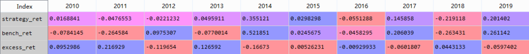
综上,是一个完整的策略回测和评价过程,当然实际操作中还有许多需要细化的地方,仅供参考,欢迎指正!